Quadratic Deep Networks in Keras

Apr 20, 2021

quad_perceptron

The past couple of months I have been scrimmaging through dozens of papers for the final research project of my degree. During this time, I have happened across several papers most of which were not directly related to my project but have kindled my interest. So I went ahead and implemented them. Some of these I found really informative In this series of posts shall share all of these small secrets that I have discovered and any others I may discover in the future, that may be of help to you for your next big project. Today's topic is Quadratic Deep Networks

A Gentle Recap of Neural Networks

The idea of Neural Networks is contrived from the biological process by which our Nervous System reacts to impulses from the external environment. An impulse triggers a neuro-chemical reaction in the axon of the neuron which then decides whether to transmit a modified signal to the next neuron (fire) or not (not fire). This binary rule of either firing or not firing based on several factors is called the All or None rule. Similar to a biological neuron, a perceptron (unit of an Artifical Neural Network) is composed of some weights $w_i$ and biases $b_i$ that determine how the input signal $x_i$ is modified and finally an activation function $\phi$ that decides whether or not to fire the modified signal

$s_i = \phi(w_i * x_i + b_i)$

However, unlike a biological neural network the purpose of an artifical neural network is not to model the human nervous system but to act as a function approximator. The analogy comes from the fact that in a way, the human cognition system can be thought of as being just one giant, enormously powerful and complex function approximator. But that is for your CS or philosophy professor to explain so I'll leave it at that.

Shortcoming of the traditional neuron

Although the idea of a neuron stems from the biological make up of our being, it is not used as such. We mostly use neural networks for classifying pictures of cats and dogs or predicting the winningest choices for your next Dream 11 Team (that's cheating btw). Underneath the pretty looking hood, it's all just math-y things with math-y equations and formulas. So to understand how a neuron works, we have to look at what a single neuron is doing. Suppose you have to model an equation $f(x) = 10x + 2$ . What would be the most optimal weights and biases by which you can model the given equation and how many neurons do you need? Easy, right? Just 1 neuron and the weights and biases are $w_1 = 10$ and $b_1 = 2$ so the final model $g(x)$ for $f(x)$ should stands as,

$g(x) = w_1x + b_1 = f(x)$

Now imagine a more complex equation, say a quadratic equation or a cubic equation. It should be evident that a single neuron cannot effectively model such an equation. In fact, it has been proven that the classical model of perceptron, which we have been following, fails spectacularly when it comes to even simple logical equations like the OR Gate or the NOR gate. The reason is apparent once you realise that the neuron only models equations that bear resemble to the equation for a line. It has also been proved beyond doubt that for modeling more complex tasks a Deep Neural Network is the way to go. A Deep Neural Network is basically just a stack of many layers each of which in turn contains many neurons. This has been shown to be effective in a large number of tasks ranging from modeling mathematical equations to driving cars automatically.

Quadratic Model of Perceptron

The Quadratic Model of Perceptron is a novel model that improves upon the classical perceptron model. It is introduced in the paper Universal Approximation with Quadratic Deep Networks (Fan et al , 2018). In this blog post, we will implement this model using the Tensorflow 2.4.1 Keras library. Note that this is the Tensorflow version that has been used to run the code blocks below but almost any version from the past couple of years should be good to go.

Recall that the model for a classical perceptron is,

$s_i = \phi(w_i * x_i + b_i)$

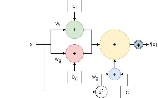
In comparison, the model for a Quadratic perceptron is,

$s_i = \phi( (w_rx^T + b_r)(w_gx^T + b_g) + w_b(x^2)^T + c )$

[refer to equation 1, Fan et al , 2018]

which is implemented in code as below -

import tensorflow as tf
from tensorflow.keras layers import Layer
from tensorflow.python eager import context
from tensorflow.keras import initializers, activations

class QuadDense(Layer):
    def __init__(self, units, activation=None, **kwargs):
        self.units = int(units) if not isinstance(units, int) else units
        self.activation = activations.get(activation)
        super(QuadDense, self).__init__(**kwargs)
    def build(self, input_shape):
        last_dim = input_shape[-1]
        self.w_r = self.add_weight(shape=[last_dim, self.units], initializer='normal', name='w_r', trainable=True)
        self.w_g = self.add_weight(shape=[last_dim, self.units], initializer='normal', name='w_g', trainable=True)
        self.w_b = self.add_weight(shape=[last_dim, self.units], initializer='normal', name='w_b', trainable=True)
        self.b_r = self.add_weight(shape=[self.units,], initializer='normal', name='b_r', trainable=True)
        self.b_g = self.add_weight(shape=[self.units,], initializer='normal', name='b_g', trainable=True)
        self.c = self.add_weight(shape=[self.units,], initializer='normal', name='c', trainable=True)
        self.built = True
  
    def apply_weight(self, x, w):
        rank = x.shape.rank
        if rank == 2 or rank is None:
            if isinstance(x, tf.sparse.SparseTensor):
                outputs = tf.sparse.sparse_dense_matmul(x, w)
            else:
                outputs = tf.linalg.matmul(x, w)
        else:
            outputs = tf.tensordot(x, w, [[rank - 1], [0]])
            if not context.executing_eagerly():
                shape = x.shape.as_list()
                output_shape = shape[:-1] + [w.shape[-1]]
                outputs.set_shape(output_shape)
        return outputs

    def call(self, x):
        x_r = self.apply_weight(x, self.w_r) + self.b_r
        x_g = self.apply_weight(x, self.w_g) + self.b_g
        x_b = self.apply_weight(x**2, self.w_b)
        x = tf.multiply(x_r, x_g) + x_b + self.c
        if not (self.activation is None):
            x = self.activation(x)
        return x

Example Dataset - The MNIST Fashion Dataset

The MNIST Fashion Dataset is a particularly hard dataset to model. We will use the AutoEncoder Architecture to design a model for this dataset. This part is not written by me and infact, is taken from the Keras Blog as is with some minor modifications.

Loading the Dataset

First we will load the dataset into memory.

import matplotlib.pyplot as plt
import numpy as np
import pandas as pd

from sklearn.metrics import accuracy_score, precision_score, recall_score
from sklearn.model_selection import train_test_split
from tensorflow.keras import layers, losses, Model, Input
from tensorflow.keras.datasets import fashion_mnist

(x_train, _), (x_test, _) = fashion_mnist.load_data()

x_train = x_train.astype('float32') / 255 
x_test = x_test.astype('float32') / 255 

print ('############ DATASET: fashion_mnist ############')
print ('train shape: ', x_train.shape)
print ('test shape: ', x_test.shape)

############ DATASET: fashion_mnist ############

train shape: (60000, 28, 28)

test shape: (10000, 28, 28)

Defining Hyper-parameters

Then we will define some Hyper-parameters. The LATENT_DIM hyper-parameter represents the dimensionality of the encoded input representation and can chosen arbitrarily We choose to use the LATENT_DIM value, and values of all the other hyper-parameters, as prescribed in the official blog post.

LATENT_DIM = 64
EPOCHS = 10
BATCH_SIZE = 32

Classical Dense Layer-based AutoEncoder

The following code block is the typical AutoEncoder model based on the classical model of the perceptron. The Dense layer is a Keras Layer corresponding to the classical version of our QuadDense implementation.

class DenseAutoEncoder(Model):
    def __init__(self, latent_dim):
        super(DenseAutoEncoder, self).__init__()
        self.latent_dim = latent_dim   
        self.encoder = tf.keras.Sequential([
          layers.Flatten(),
          layers.Dense(latent_dim, activation='relu'),
        ])
        self.decoder = tf.keras.Sequential([
          layers.Dense(784, activation='sigmoid'),
          layers.Reshape((28, 28))
        ])

    def call(self, x):
        encoded = self.encoder(x)
        decoded = self.decoder(encoded)
        return decoded

dense_autoencoder = DenseAutoEncoder(LATENT_DIM)
dense_autoencoder.compile(optimizer='adam', loss=losses.MeanSquaredError(), metrics=['accuracy'])
dense_ae_hist = dense_autoencoder.fit(x_train, x_train,
                                        epochs=EPOCHS,
                                        shuffle=True,
                                        batch_size=BATCH_SIZE,
                                        validation_data=(x_test, x_test))

Quadratic Dense Layer-based AutoEncoder

Now let us run the same task but with another AutoEncoder model which is essentially the same as the above model except that instead of the classical Dense layers, we use the QuadDense Layer that we have implemented before.

class QuadDenseAutoEncoder(Model):
    def __init__(self, latent_dim):
        super(QuadDenseAutoEncoder, self).__init__()
        self.latent_dim = latent_dim   
        self.encoder = tf.keras.Sequential([
          layers.Flatten(),
          QuadDense(latent_dim, activation='relu'),
        ])
        self.decoder = tf.keras.Sequential([
          QuadDense(784, activation='sigmoid'),
          layers.Reshape((28, 28))
        ])

    def call(self, x):
        encoded = self.encoder(x)
        decoded = self.decoder(encoded)
        return decoded

quad_dense_autoencoder = QuadDenseAutoEncoder(LATENT_DIM)
quad_dense_autoencoder.compile(optimizer='adam', loss=losses.MeanSquaredError(), metrics=['accuracy'])
quad_ae_hist = quad_dense_autoencoder.fit(x_train, x_train,
                                            epochs=EPOCHS,
                                            batch_size=BATCH_SIZE,
                                            shuffle=True,
                                            validation_data=(x_test, x_test))

Comparison of Results

Let us compare the results of the classical Dense Layer-based AutoEncoder and the novel QuadDense Layer-based AutoEncoder.

from matplotlib import pyplot as plt
%matplotlib inline

fig, axs = plt.subplots(2, 1, figsize=(8,10))

axs[0].plot(dense_ae_hist.history['val_accuracy'])
axs[0].plot(quad_ae_hist.history['val_accuracy'])
axs[0].set_title('Comparison of Model Validation Accuracy')
axs[0].set(xlabel='epoch', ylabel='accuracy')

axs[1].plot(dense_ae_hist.history['val_loss'])
axs[1].plot(quad_ae_hist.history['val_loss'])
axs[1].set_title('Comparison of Model Validation Loss (MSE)')
axs[1].set(xlabel='epoch', ylabel='loss')

axs[0].legend(['Accuracy: Dense AutoEncoder', 'Accuracy: Quadratic Dense AutoEncoder'], loc='upper left')
axs[0].legend(['MSE Loss: Dense AutoEncoder', 'MSE Loss: Quadratic Dense AutoEncoder'], loc='upper left')

plt.show()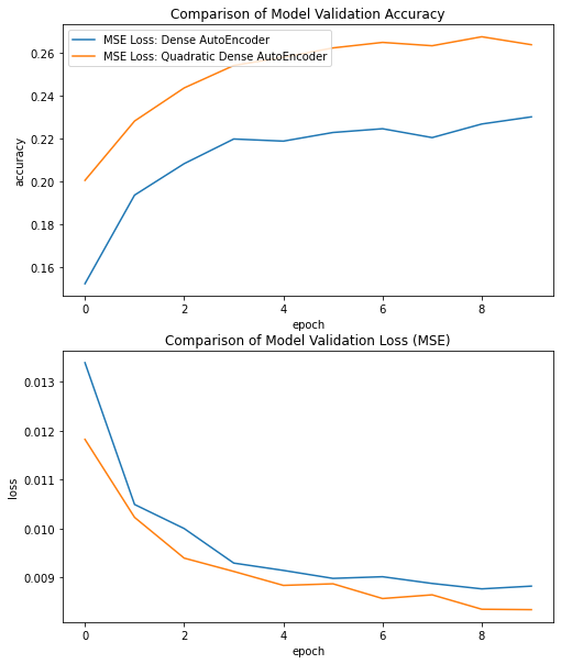

results

It is clear that the Quadratic Dense Layer-based Auto-Encoder beat the classical AutoEncoder by a significant margin. In fact, for almost all models (and especially the Auto-Encoder models since they heavily rely on the Dense Layer) the Quadratic Dense Layer outperforms the classical Dense Layer.

Conclusion

It is worth mentioning that this is not true, however, for all cases. In some cases where the classical Dense Neural Network is already sufficiently capable of modeling the target dataset, the Quadratic Dense Layer provides almost insignificant or sometimes no improvement. But in no cases have I found that using the Quadratic Dense Layer reduces the accuracy or increases the loss. In short, try the Quadratic Dense Layers when your target dataset is fairly complex and your model modest-to-heavily relies on Dense Layers. This may give you an added boost to your model in the best case and show no improvements in the worst case.

Thanks for reading! Happy coding 😊